12 April 2014

A Beginner’s Tutorial for knitr

My first homework assignment for my Machine Learning class was a mess. I was copying and pasting code into my LaTeX file, I was manually running and saving graphs in R as PNGs and PDFs.

There has to be an easier way of doing this, I thought. A search or two later and I learned about knitr. I have never looked back and completely love it.

If this sounds like you or if you are upset with Sweave, then you really need to check out knitr (GitHub Source).

Also, if you don’t do your homework in LaTeX, you’re really missing out.

Foreword

Yihui's book

This is meant to be a short intro to knitr; it isn’t meant to be comprehensive.

If you wish to learn more about knitr in depth, check out Yihui Xie’s book, Dynamic Documents with R and knitr. He’s the creator of knitr and has written a really, really excellent book on it.

On a sidenote, he got his PhD in Statistics from Iowa State University where I am finishing up my Bachelor’s degree.

Together he and Hadley Wickham both graduated from ISU and both have contributed a whole lot to the R community.

Getting Started

First you’ll need to install knitr from CRAN if you don’t already have it. This can be done by launching R and running:

install.packages('knitr', dependencies = TRUE)

You can verify that it has been installed by running:

library('knitr')

If you don’t get any errors, you’re good to go! If you do get errors, check out the knitr FAQ to see if there are any solutions.

Adding R Code

Adding R code to a LaTeX document is as easy as adding a chunk. A chunk is just what knitr calls a section of R code. Each chunk can have its own options to configure how it is rendered.

A simple example chunk in LaTeX looks like this:

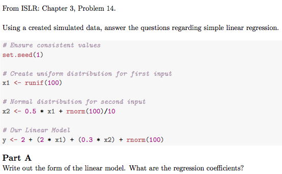
From ISLR: Chapter 3, Problem 14.

Using a created simulated data, answer the questions regarding simple
linear regression.

<<>>=
# Ensure consistent values
set.seed(1)

# Create uniform distribution for first input
x1 <- runif(100)

# Normal distribution for second input
x2 <- 0.5 * x1 + rnorm(100) / 10

# Our Linear Model
y <- 2 + (2 * x1) + (.3 * x2) + rnorm(100)
@

\part

Write out the form of the linear model. What are the regression
coefficients?

Which will end up being rendered like this:

Basic chunk example

Basic Chunk Options

If we want to just show code without seeing the results, we can do that by adding eval=FALSE to the chunk options. Like so:

<<eval=FALSE>>=
# This code is just shown, it isn't ran
x1 <- runif(100)
@

As you can see, all the options go within the angle brackets.

Another common one that I use for things such as imports is to set echo=FALSE. This will hide the code but still evaluate it.

There are a ton of other chunk options that allow you to completely fine tune how to handle the R code in your documents.

Referencing R Variables

Since the R code is evaluated as you compile your document, you can include variables in your normal LaTeX.

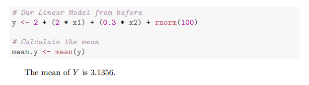
Let’s say you wanted to compute the mean() of y, store it in a variable and then include it in output below it. It would look like this:

<<>>=
# Our Linear Model from before
y <- 2 + (2 * x1) + (.3 * x2) + rnorm(100)

# Calculate the mean
mean.y <- mean(y)
@

The mean of \(Y\) is \(\Sexpr{mean.y}\).

The output is in the image below. This makes it really, really easy to keep info up to date and not have to worry about re-computing values.

You can put any R code in the \Sexpr{}. More info about that can be found under the Inline output section on the knitr Output page.

Values from R in LaTeX

Figures

This is the most indespensible feature of knitr. It is capable of automatically evaluating the R code and including any graphs that are output.

Let’s go back to our simple linear model. If we add this to our LaTeX document:

Which checks out with our value.  This suggests that \(X_1\) and \(X_2\) are
pretty colinear. Let's visualize this by using a scatter plot:

<<p1b, fig.pos="H", fig.height=4, fig.cap="Correlation of given predictors.">>=
plot(x1, x2,
     main = 'Correlation of X1 and X2',
     xlab = 'X1',
     ylab = 'X2')
@

Then we get this as the output:

Simple figure

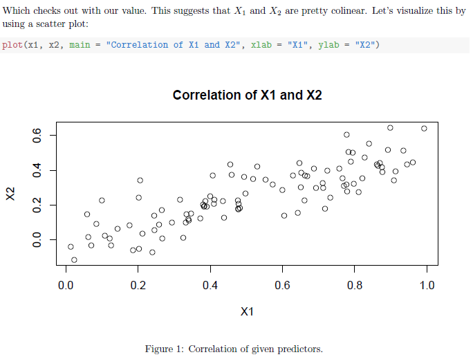
We don’t have to worry about outputting our image, saving it, then adding it to LaTeX. Instead, knitr handles all of that for us.

We are using a few more chunk options as well. The first, p1b, is just a label that allows us to refer to it by name.

Next we are using the option fig.pos="H", this tells knitr to include it with a certain position. These options are given by LaTeX’s figure environment.

Then we set a height for the figure as well as giving it a caption. As you can see, the caption ends up at the bottom of the figure.

Once again, these figure chunk options can be found on the same chunk options page.

Running knitr

Before typesetting the LaTeX code, you need to first run it through knitr. My preferred way to do this is by running the following:

$ Rscript -e "library(knitr); knit('./file-here.Rnw')"

Where file-here.Rnw points to your knitr file. This will automatically output the accompanying formatted output. So for this example, we will then get a file called file-here.tex which will be all ready to typeset.

You can then run this through LaTeX anyway you wish. However, I like to automate things because it allows me to seamlessly edit files. I’ll talk about that next.

Seamless Editing

I do all of my editing in Vim so one of the things that I like is automatic typesetting of LaTeX when I save.

I have the following saved in my ~/.latexmkrc file:

if ($^O eq 'darwin') {
    # Open Skim when using OS X
    $pdf_previewer = "open -a Skim.app";
} else {
    # Open Mint's default pdf viewers
    $pdf_previewer = "mate-open";
}

This launches my preferred PDF viewer depending on the system that I’m on. All I need to run this is to run:

$ latexmk -pdf -pvc solution.tex

The -pvc is a special option for latexmk. It tells the system to run a file previewer and continously update the output whenever changes are made to the source file, solution.tex.

Watching a knitr File

Since latexmk works great for watching tex files, I wrote up a little script that I’ve called knitr that I place on my $PATH. It allows me to run:

$ knitr file-here.Rnw

And will automatically run knitr whenever the source file updates. It uses Ruby’s kicker to watch for a file change and run a specific command.

The entire source can be found here but here is the basic idea:

FILE="${1}"

KNITR="echo \"Rerunning knitr...\"; Rscript -e \"library(knitr); knit('./${FILE}')\""

echo "Watching ${FILE}..."
kicker -e "${KNITR}" ${FILE}

Conclusion

Together with these scripts and knitr, I’m able to edit a LaTeX + R file and have it constantly updated and formatted. When I keep my PDF viewer open, I can see my document evolve right in front of me.

knitr makes working on Statistics and Machine Learning a breeze. I can’t imagine trying to work without it.

Do you use knitr and have some feedback? Feel free to send me an email me or Tweet at me on Twitter: @HopefulJosh. I’d love to learn more or talk.